How to Create a Gantt Chart in Google Sheets

Google Sheets is a great alternative if you don’t want to pay for Microsoft Excel. Google Sheets is a spreadsheet program that comes free with the Google Docs Editor Suite. Unlike Excel, Google Sheets is also cloud-based, which means you can share your spreadsheets with anyone and collaborate on them at the same time.

One of the most popular uses of Google Sheets is as a project management tool, but Google Sheets doesn’t have the ability to create a Gantt chart in its chart editor. However, there are workarounds to do this so you can keep track of your projects. We’ll show you how.

When to use a Gantt chart

Gantt charts are used by project managers in virtually every major project management methodology. While essentially horizontal bar charts, Gantt charts are a great way to visualize progress and are typically used to break down large projects into manageable chunks.

Gantt charts are also useful when you need to report on specific milestones for your project or when your project involves many people.

How to create a Gantt Chart in Google Sheets

Unfortunately, there isn’t a button you can press in Google Sheets to create a Gantt chart for you, but that shouldn’t stop you from creating a working project management board in Google Sheets. If you want to create a Gantt chart in Sheets, there are two options.

1. The easy way to create a Gantt chart in spreadsheets – templates

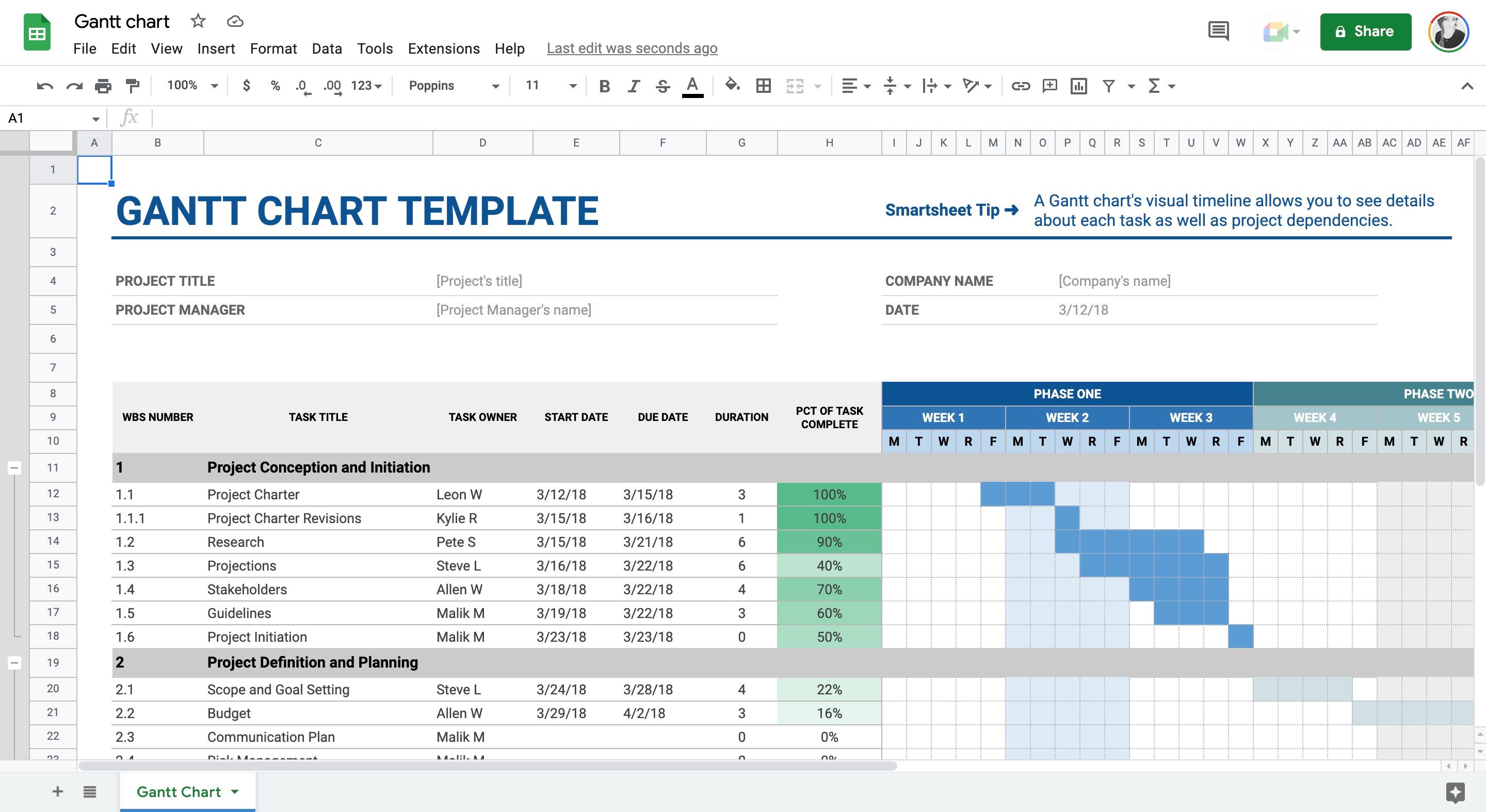
The easiest way to create a Gantt chart in Google Sheets is with a pre-made template. Templates do most of the hard work for you, so you can focus on refining your Gantt chart instead of creating it from scratch.

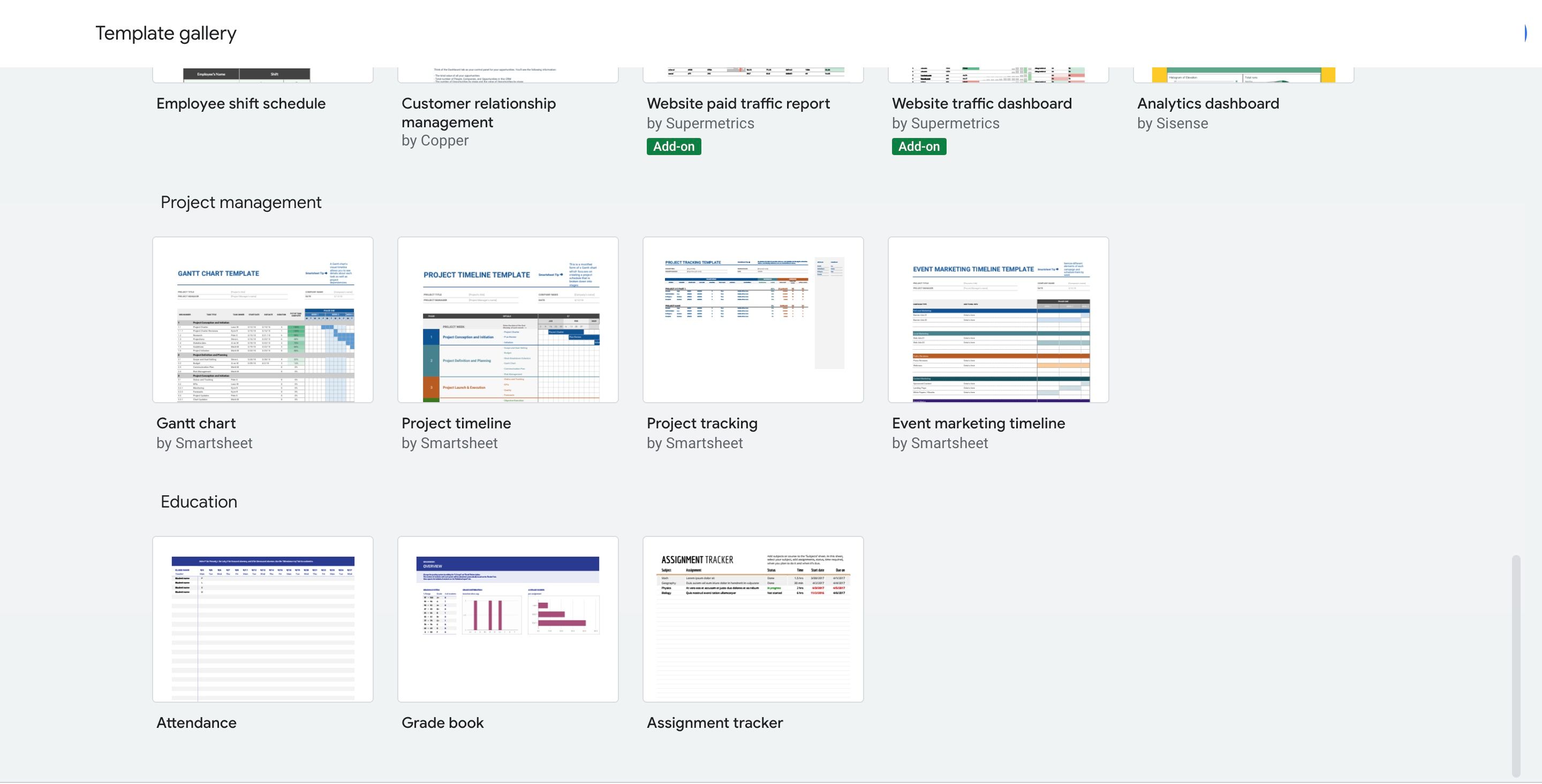
You can find a Gantt chart template on your Google Drive by creating a new Google Sheet from a template. To do this, open your Google Drive and select + Newthen select Google Spreadsheetand then select From a template.

This opens the Template gallery. Inside the Template galleryscroll down to the titled section project managementand you will find a template titled Smartsheet Gantt chart.

If you don’t see the Smartsheet template above, or if it looks a bit overwhelming, try this free Gantt chart template from Forbes Advisor. It’s much easier but saves you a lot of time.

2. Creating a Gantt Chart from Scratch in Google Sheets

If you don’t want to use a template to create a Gantt chart in Google Sheets, you can create one from scratch. How to create a Gantt chart with a stacked bar chart in Google Sheets.

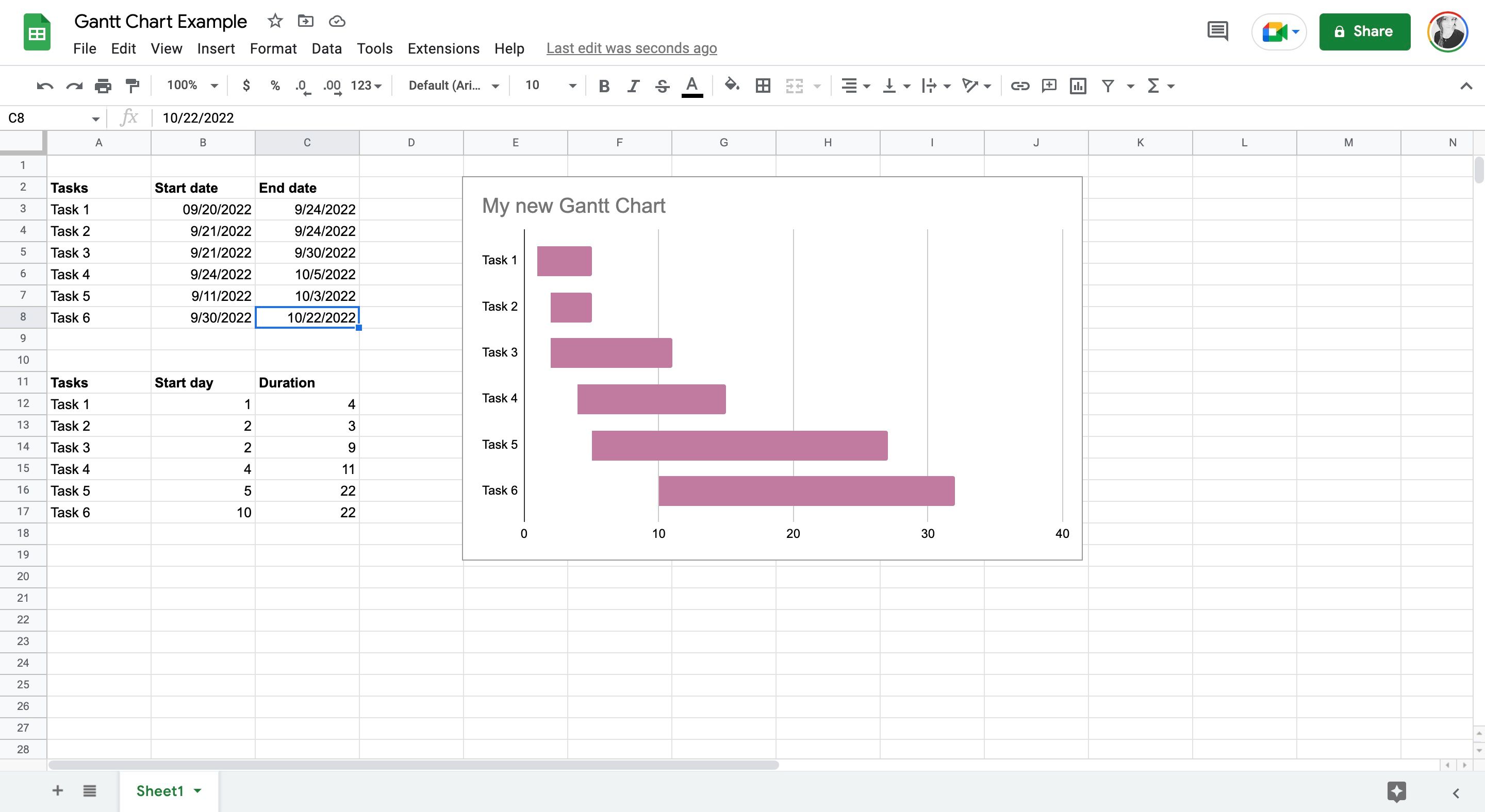
Enter your project details into a new Google Sheet. This must include the name of each task and the start and end dates.

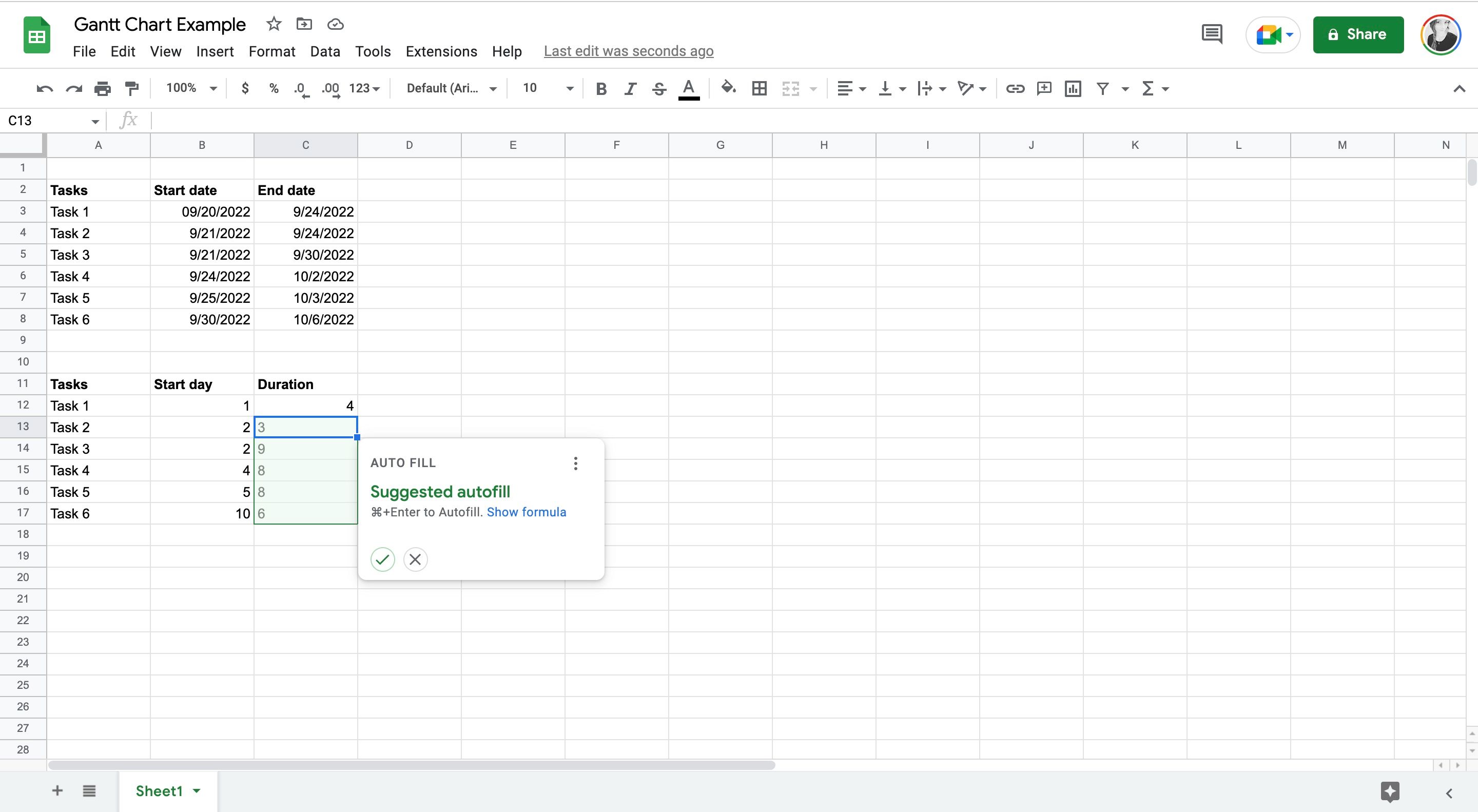
Next you need to calculate the duration of each task. Use a simple Google Sheet formula to make calculating the duration of each task easy. A formula also ensures that any changes made to the start and end dates of your tasks are reflected in your finished Gantt chart.

Use this formula to calculate the duration of each task: End Date – Start Date = Duration.

For example, if your start date is in column B, row three and your end date is in column C, row three, use the formula: =sum(C3-B3). You only have to write this formula once and then you can drag it using the little blue box in the corner. This will apply the formula to all selected dates.

If you’re struggling with the basics of Google Sheets, check out some of our other tutorials.

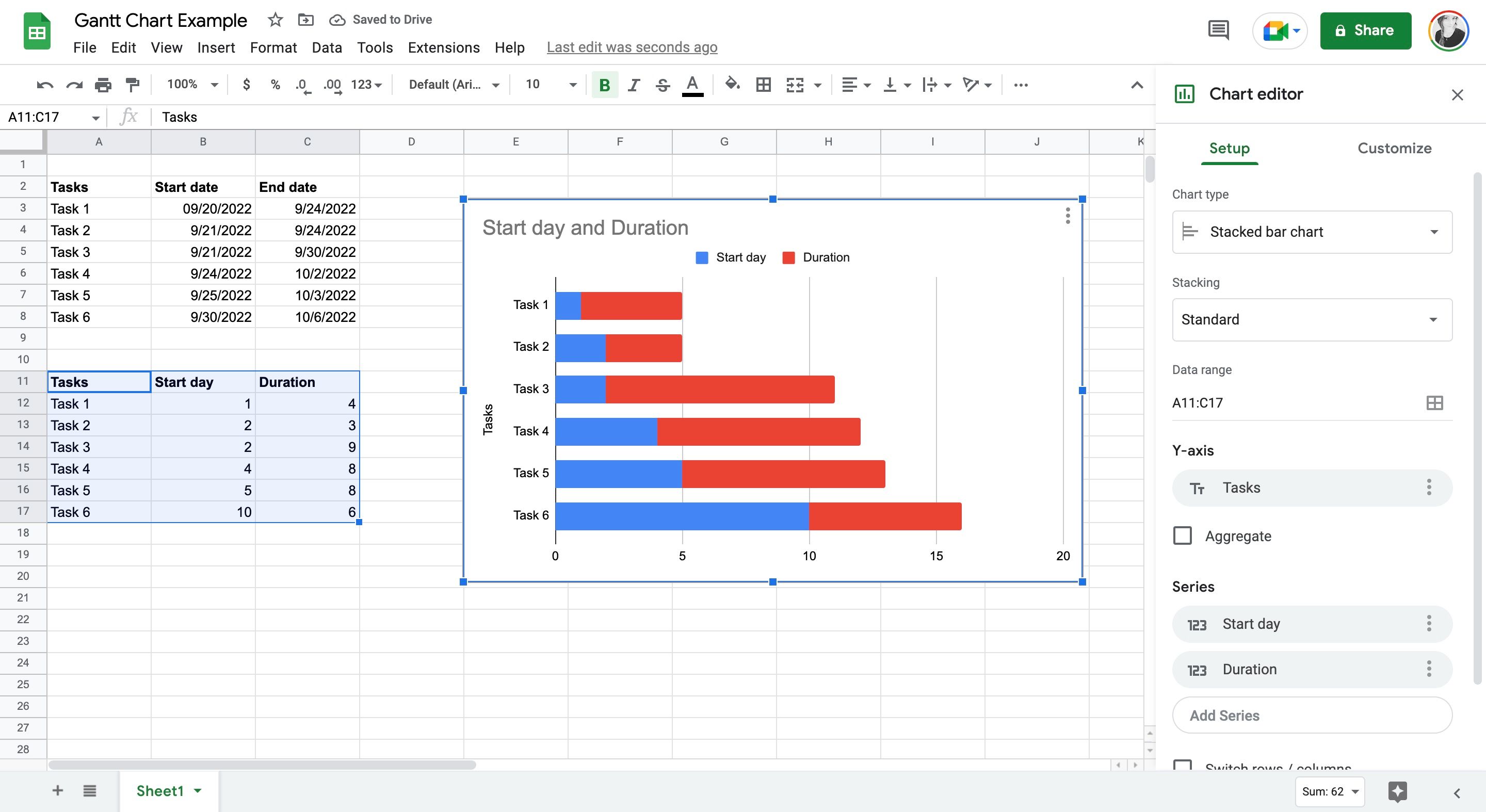
Next you need to create a stacked bar chart. To do this, it helps to have a second table with your task names, the day they start, and their duration.

Highlight your second spreadsheet with your task names, start day, and duration, then select insertionand then diagram. If Google Sheets didn’t automatically select a stacked bar chart, you can manually change the chart type.

Right now you have a stacked bar chart, but as you can see it doesn’t look like a Gantt chart. To make this bar chart look and feel more like a Gantt chart, you need to make some changes to your chart settings.

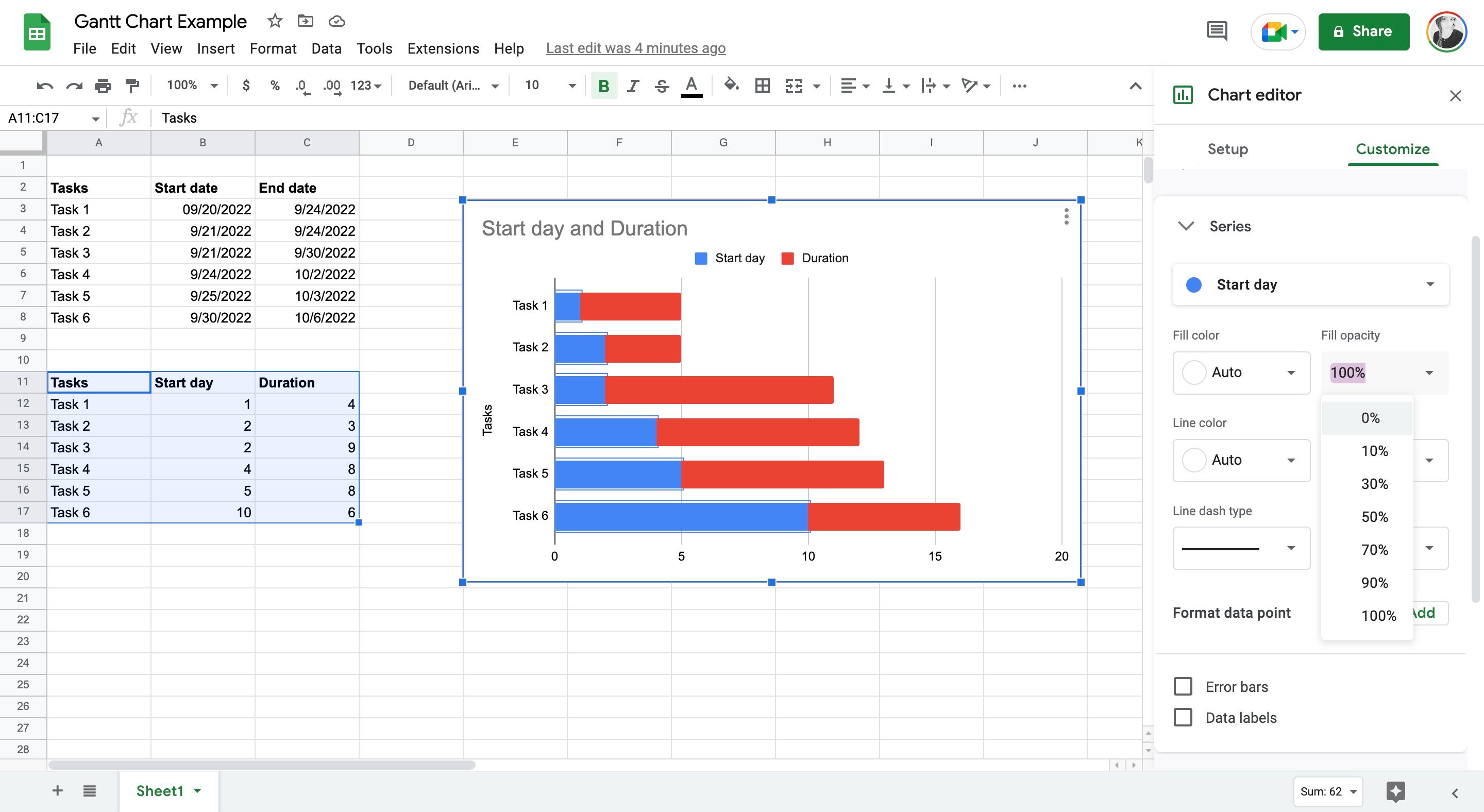
First you need to remove the blue part of the stacked bars, which represents the start day for each task. In order to do this, double click the diagram to open the Diagram Editor and then click on the blue part of the chart.

This opens the series settings. You can’t completely erase the blue bars, but you can make them invisible by changing their opacity from 100% to 0%.

Now you can’t see them, but they still keep the important red parts of your bar chart where they need to be.

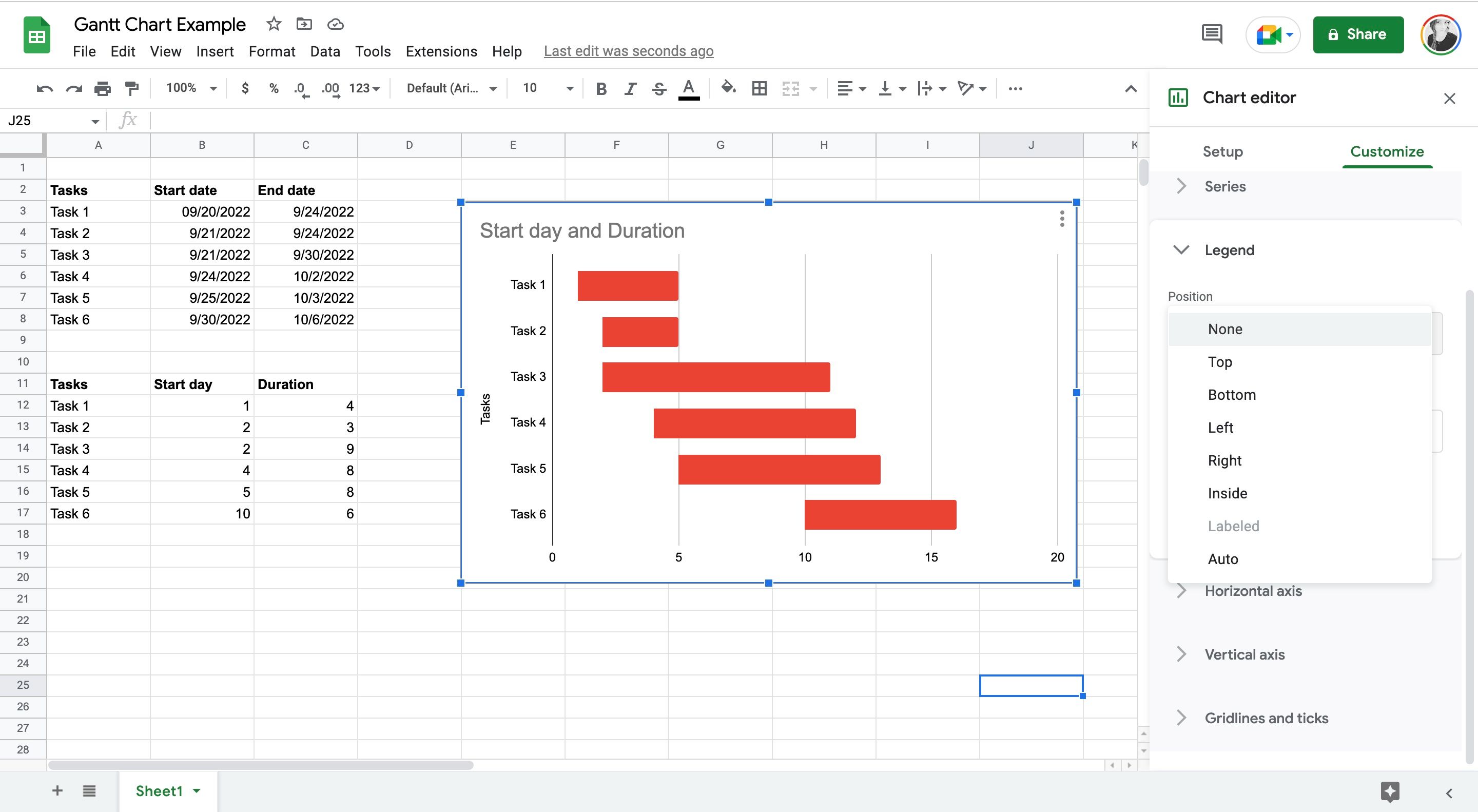
Next you need to remove the legend from your chart. Click on the labels at the top of your chart and then change their position from top to none. You can also clear the legend by tapping Clear key on your keyboard.

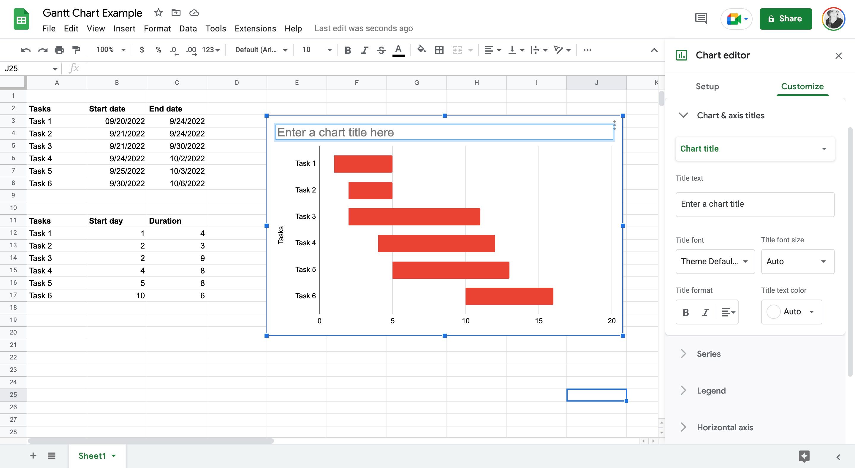
Finally, give your Gantt chart a title of double click the existing title and make your changes. You can also clear the axis title by clicking and then typing on it Clear on your keyboard.

If you’re not a red fan, then change the color of the red bars around click one of them and then select a new one fill color.

Now you have a Gantt chart that updates automatically whenever you change the start or end date of a specific task.

Manage projects in Google Sheets

You now know how to create a Gantt chart in Google Sheets. Whether you’re using a template or creating a Gantt chart from scratch, you’re now ready to start managing a project with Google Sheets.

Project management tools like Asana can create Gantt charts for you, but they’re also paid programs. Google Sheets is completely free, so if you don’t have a big project management software budget, it’s worth learning how to manage a project in Google Drive.