How to sort your data in Google Sheets

September 17, 2022 Abraham Smith

Google Sheets is a remarkably powerful and handy tool for collecting and analyzing data, but sometimes it can be difficult to understand what that raw data means. One of the best ways to see the big picture is to sort it to bring the most important information to the top and show which value is the largest or smallest compared to the rest.

It is not surprising that Google Sheets has a powerful search function. It’s also easy to sort data in Google Sheets, but some concepts need to be clear to get the best result and get the most valuable insights. With a few tips, you can quickly master sorting by one or more columns and access different views to better understand the meaning of the data.

How to quickly sort a simple sheet

Sorting a Google Sheet by a single column is quick and easy. For example, given a table of foods that are good sources of protein, you might want to sort by name, serving size, or amount of protein. Here’s how.

Step 1: Hover over the column you want to sort by and select it down arrow that seems to open a menu of options.

Options appear after selecting a column's triangle menu.

Step 2: A little more than halfway down the menu are the sorting options. Choose Sort the sheets from A to Z to sort the entire sheet so that the selected column of text is in alphabetical order. Sort sheet Z to A places this column in reverse alphabetical order.

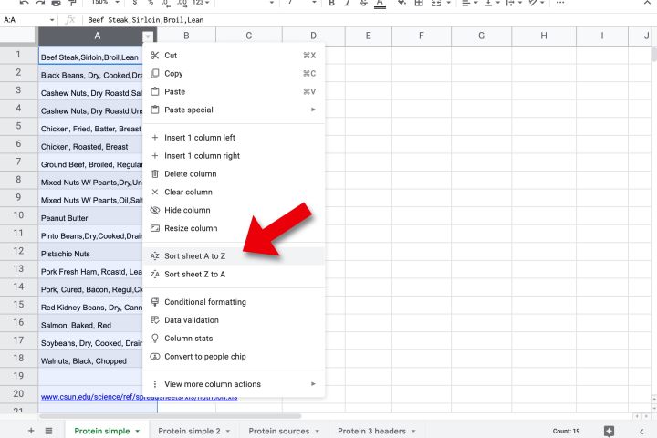
Step 3: To sort a numeric column, do the same. Choose Sort the sheets from A to Z for a low to high order of numerical values or Sort sheet Z to A to see the highest values above.

The same sorting options are available for numbers.

Step 4: Regardless of which column is sorted, the information from all other columns in the sheet is shifted to keep the same order. In our example, a cup of walnuts still shows 30 grams and a 2.5-ounce steak has 22 grams of protein.

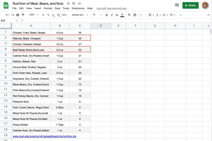
Sorting a sheet by a column keeps the row data aligned.

Step 5: If a numeric column shows values in more than one unit, the sort will not return the expected result. In our example, the Google Sheet on protein sources, the Serving Size column includes cups, ounces, tablespoons, and slices. Units are ignored by the built-in sorter conversion, so 1 cup is incorrectly treated as being less than 3 ounces. The best solution is to convert the data to use only one unit per column.

Google Sheets doesn't take units into account when sorting.

Sorting a sheet with headers

The quick sort method described above is convenient; However, it does not work as expected when the sheet contains headers. By default, when you sort the entire sheet, all rows are included, which allows for headings and units to be mixed in with the data. Google Sheets can lock cells so they can’t be changed, but it’s also possible to lock one or more rows at the top so headings aren’t confused with your information.

Step 1: To freeze the header position, select Google Sheets outlook Menu. Instead of using your browser’s view menu, open the outlook Menu at the top of the opened web page. Then select the Freeze option and choose 1st row or 2 rowsdepending on the number of headers in your sheet.

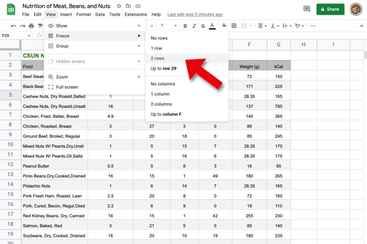
Freeze a line or two to lock the headers.

Step 2: If there are more headers, it is possible to freeze more rows. Just select a cell in the bottom header row and then select Freezethen Up to line X in the View* menu, where X is the line number.

Step 3: After freezing headers, a thick gray line appears showing where the split is occurring. A sheet can then be sorted using the column menus Sort the sheets from A to Z or Sort sheet Z to A Possibility. This keeps the headers at the top of your Google Sheet while rearranging your data into a more useful spreadsheet.

Column menu can sort while keeping frozen headers.

Sort by more than one column

A single-column sort is quick and convenient, but often when comparing numbers, more than one variable needs to be considered. In our example, you may be the least interested in fat, but you also want to get more protein. It’s easy with a sorting area.

Step 1: Select the cells you want to sort, including a header. This is done quickly by selecting and then holding the cell in the top left control Key (command key on a Mac) and press the right arrow to select the entire width of the table.

Use Ctrl+Right Arrow to select a horizontal range

Step 2: The same can be achieved by selecting full height and holding controland press the down arrow. Now the entire data table is selected.

Use Ctrl+Right Arrow and then Ctrl+Down Arrow to select an area.

Step 3: From Google Sheets Data menu, choose sort area > Advanced range sorting options.

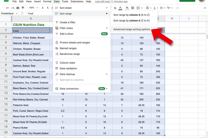
Google Sheets advanced sorting is in the data menu

Step 4: A window opens in which you can select several sorting columns. If your sorting pane includes a header, check the box next to it Data has a header.

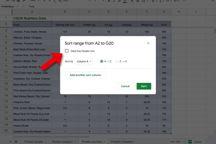
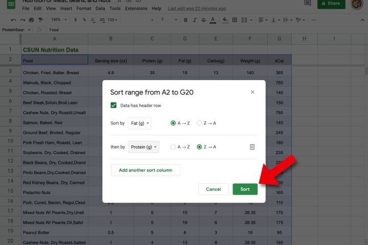
You can see the header names if this box is checked

Step 5: That sort by -Field now displays the names of your header columns instead of letting you select columns by their letter designation. Choose the primary sorting column – for example fat (g) – and make sure AZ is selected for the sort order.

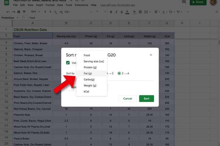
If the header is activated, the names are displayed in the Sort by field.

Step 6: Select the Add another button to sort columns to have a secondary type, such as B. Protein. It is possible to add as many sort columns as you like before selecting them sort by click to view the results.

You can add more sort columns before sorting your data.

Save a range of data

Instead of selecting a range each time you want to reorder it, you can save the table as a named range.

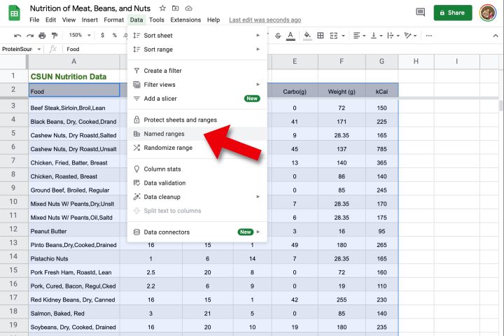
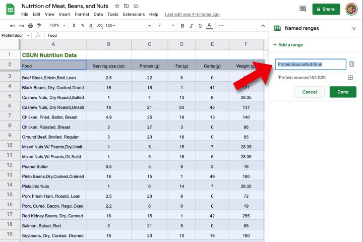
Step 1: Select the range of data you want to save for easier access, then select Named Areas from Google Sheets Data Menu.

Step 2: A pane will open on the right where you can enter a name for this pane.

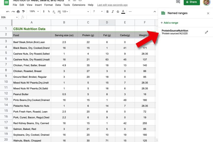
Step 3: That Named Areas The panel stays open and you can reselect the entire range by selecting it in this panel.

Select a named range to select all of its data.

Save a sort view

It is also possible to save more than one advanced sort for easy access later. This allows you to switch between different views when you need to create a presentation or analyze information from different angles. This is possible by creating a Google Sheets filter view.

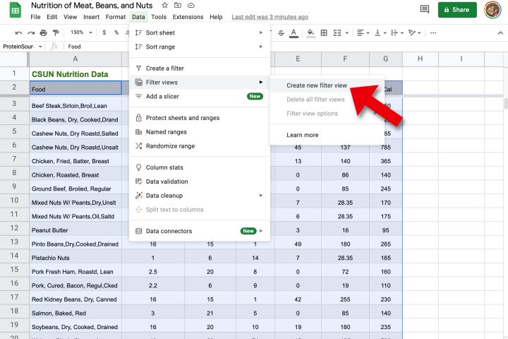
Step 1: Select the range of data you want to sort, and then select Create new filter view of the filter Submenu in Google Sheets Data Menu.

Create a filter view to save advanced sorts.

Step 2: A new bar with filter view options will appear at the top of the sheet. Select the name field and enter a name for this filter view, e.g. B. “Low Fat/High Protein”.

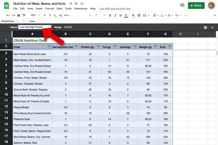
Filter views can be named in a way that is easy to remember

Step 3: The name of each header column now includes a sort menu on the right. Using our example data, select the protein Sort menu and then select Sort ZA to place the highest values at the top.

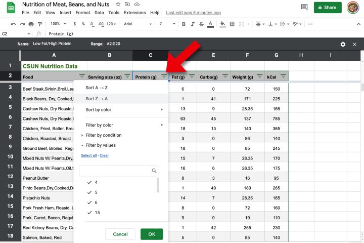
Step 4: Repeat this process on the Fat Sort menu, but select Sort A-Z to show the lowest values first. This new filter view shows a low fat variety as a top priority and high protein as a secondary consideration.

Multiple columns can be sorted using a filter view.

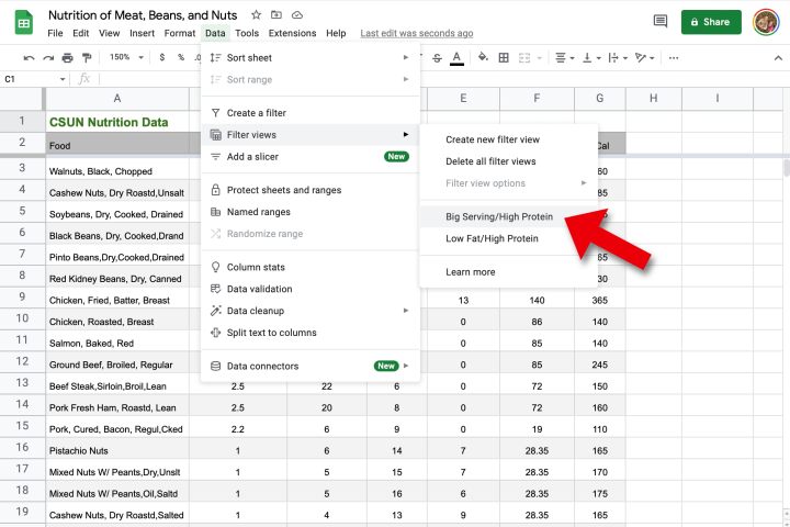
Step 5: You can create more filter views in the same way and use as many sorting columns as you like. To load a filter view, open the Data menu, select filter viewsand then select the view you want.

Filter views can be loaded from the Data menu.

How to share a sorted Google Sheet

Google Sheets is readily available to anyone with an internet connection, making it a great tool for sharing information with others.

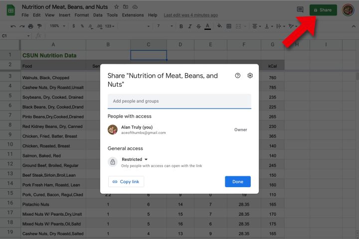
Step 1: Sorted spreadsheets can be shared by selecting the big green Split button in the top right corner.

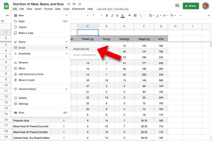
The share button makes it easy to collaborate with others.

Step 2: It’s also possible to download a Google Sheet to share via email or print it out to send in the mail.

You can also share a Google Sheet via email.

Google Sheets offers multiple ways to sort data, and this can make a world of difference when you’re trying to analyze a complicated dataset. For more information, check out our complete beginner’s guide on how to use Google Sheets.

We also have a guide that explains how to create graphs and charts in Google Sheets, a great way to display data in an easy-to-understand visual form.

unugtp